A Real Estate View Should Tell You What Would Change It

Clearer assumptions, visible sources and comparable calculations make research more useful in an allocation decision.

Before an investment committee advances a real estate opportunity, it should know which assumption could take the projected return below its required hurdle.

An attractive projected return does not answer that question. The return might come from current income, operating improvement, a more favorable sale price, or a combination of all three. Each requires different evidence. If rejecting one assumption takes the return below the required hurdle, that assumption deserves attention early in diligence.

That is what the improvements to Steuart and our forthcoming Q3 Cross-Asset Real Estate Report are intended to make easier: understanding what drives the conclusion and testing whether it survives a different view.

Steuart is the internal research engine we built to support the work William McSweeney, CFA weeney and I do at EM Capital. It helps us apply a consistent framework, examine sources and test assumptions. We remain responsible for the conclusions. For the reader, the value is in being able to inspect the inputs and challenge how we use them.

Clearer assumptions

The Q3 return build shows entry pricing, recurring capital spending, income growth, exit valuation and modeled transaction costs on a common five-year, unlevered basis. Unlevered means before the effects of borrowing. Net operating income, or NOI, is property income after operating expenses and before financing costs. Recurring capital needs still have to be funded from that income.1

Showing those terms separately makes it possible to understand what the estimate depends on. A property can have an attractive income yield and consume enough capital to leave much less cash available. Another can produce limited growth but appear compelling because the exit assumes a buyer will pay more for each dollar of income.

Neither conclusion follows from the headline return alone. Separating the terms tells an allocator where to look next.

Consider the simplified calculation below. These are hypothetical inputs, not Q3 forecasts. Both columns use the same entry income yield, capital spending, NOI-growth assumption, costs and required return. The second removes the benefit from selling at a lower capitalization rate. A cap rate expresses property income as a percentage of value; a lower cap rate means a higher price for the same income.

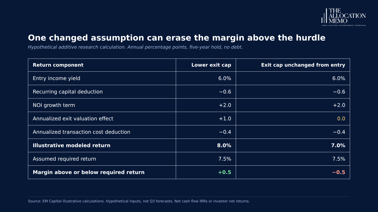
Source: EM Capital illustrative calculations. The 6.0% entry yield is reduced by recurring capital equal to 10% of entry NOI.

The first column clears the assumed hurdle by half a percentage point. Remove the one-point valuation contribution, and the second falls short by half a point. Accept only half of that contribution, and the estimate lands exactly on the hurdle, with no margin left. The operating assumptions have not deteriorated. The difference comes from what the next buyer is assumed to pay.

The next diligence task is to test the evidence for the lower exit cap. Better asset quality, a more secure income stream or a change in market pricing could justify it. Any spending needed to produce those improvements belongs in the calculation too. Holding the cap rate unchanged is a diagnostic, not a universal definition of a conservative case. But an allocator who needs that valuation benefit to meet the hurdle should understand the evidence behind it before treating the return as adequate.

This is also why the calculation's conventions matter. An additive research estimate helps compare assumptions across sectors. An investment decision requires dated cash flows, the financing structure, fees, carried interest and taxes relevant to the investor. A five-year unlevered estimate cannot be compared directly with a fund's levered net IRR simply because both are percentages.

Greater transparency

A published input becomes more useful when its source and basis are clear.

The Q3 analysis identifies whether an entry yield comes from a broker survey, a public operator's acquisition guidance or a listed-market proxy. Those inputs describe different evidence. A survey estimate is not a closed transaction. A listed REIT's implied pricing reflects a portfolio and corporate structure that may differ from the private property being considered. An appraisal at loan origination answers a different question from the price in an executed sale.1

The purpose is to make those differences visible before the reader carries a reference into underwriting. If a sector estimate uses a listed proxy because the private-market evidence is thin, the reader should know that. The next question is whether the property in front of them resembles the assets behind the reference closely enough for it to be useful.

The same discipline applies to our judgment. Q3 shows the historical sector spread used in the exit calculation and the adjustment that expresses our view. A reader can disagree with that adjustment and see what changes. The scenario comparisons also hold other assumptions, including the required return, constant while changing the exit valuation.1

That isolates a sensitivity. It does not predict that income growth, financing conditions and valuation will move independently in the real world. The report's one-for-one relationship between an assumed exit Treasury yield and the exit cap is a modeling convention. It must be judged alongside the conclusion it produces.

A consistent calculation still rests on choices about sources, periods and economic relationships. Selecting a required return is one of those choices: passing our sector hurdle does not establish that an opportunity meets your mandate. Steuart helps us apply and examine the framework; we remain responsible for the choices within it. Publishing them makes disagreement more precise. A reader can challenge the source, the assumption or the method rather than having to accept or reject the whole report.

More useful comparisons

The forthcoming report puts its main conclusions first, then connects them to the sector evidence and calculations. The intended benefit is a shorter path from a view to the assumption that supports it.

Comparability also requires care when a conclusion changes between editions. An upgrade can reflect stronger property economics, a lower entry price, a revised assumption or a changed method. Those explanations have different implications for an allocator.

Senior housing illustrates the distinction. The Q2 material placed it at Hold/Trim. The Q3 analysis we are preparing places it at Overweight. The operating case includes constrained supply and demand from an aging population, but favorable demographics were already part of the earlier thesis. They cannot, on their own, explain a new rating.3

NIC's July release provides operating support for the constructive view, describing rising occupancy alongside limited additions to supply. Q3 also updates valuation assumptions and changes the required-return method. Those changes affect the result alongside the operating evidence. The upgrade should not be read as a measure of market improvement alone.4

The revised hurdle is particularly important. The earlier framework combined a Treasury yield, a credit spread and a sector risk premium. Q3 uses the Treasury yield plus a sector premium derived from that sector's historical cap-rate spread, leaning on historical base rates to orient required rates per sub sector. That changes the benchmark the modeled return must clear. It does not establish that the underlying investment has become safer.1,3

The holding period needs the same discipline. Q3 uses five years. A comparison with a four-year calculation must reconcile the horizon: the same total exit-value change or transaction cost produces a different annual contribution when spread over a different period. The comparison needs a consistent basis before the difference can be interpreted.

Beginning with Q3, each quarterly edition will include a short change note explaining material ranking changes. It will distinguish new market evidence, revised assumptions or judgment, and methodology changes. When several causes interact, the note should say so rather than assign the entire move to whichever market narrative sounds most persuasive.

That explanation matters even when the label stays the same. A sector can remain Overweight while its margin above the hurdle narrows or its return becomes more dependent on a particular assumption. The label summarizes a view. The underlying changes determine how the reader should use it.

There is a limit to what these improvements establish. Transparent assumptions can still be wrong. More detailed calculations do not, by themselves, demonstrate better forecasting.

Our residential home-price backtests, the separate evidence on metro rent growth, and the sector return calculations answer different questions. Evidence about selecting residential markets does not validate a ranking across property sectors. The report acknowledges the limits of that cross-sector evidence. None of those exercises is a record of realized returns for an investor.1

The same boundary applies to manager diligence. Sector research can identify the assumptions worth questioning and the evidence worth requesting. It cannot establish whether a particular sponsor can execute, whether its financing survives a downside case or whether the investment's terms fit a client's constraints. Those questions still require work on the actual opportunity.

I am excited to share the official report because these changes let readers do more with our analysis. They can follow a conclusion back to its inputs, see where our judgment enters, and decide whether their own assumptions support the same view.

For an RIA or family-office team, the immediate use is to focus the next diligence discussion. In the example, the return needs at least half a point of annual valuation benefit just to meet the hurdle. Evidence supporting that benefit justifies further work. Without it, the team needs a better entry price, another supportable source of return, or a reason to direct its attention elsewhere.

A useful real estate view should leave the reader able to understand the conclusion, challenge its assumptions and identify what would change it.

Sources and calculation notes

1. EM Capital, Cross-Asset Real Estate Quarterly Report, Q3 2026, pre-release analysis reviewed September 29, 2026, 82-page version: pp. 6, 68–70 and 73–74 for scenarios, sources, required returns and the return build; pp. 28–29 and 68 for validation limits. Forward-looking research estimates, not realized investment returns.

2. The exhibit is hypothetical and uses the report's additive structure. Lower exit cap = 6.00% ÷ 1.01⁵ = 5.708794...%, displayed as approximately 5.71%. The annual valuation term is the fifth root of the ratio of entry to exit cap, less one, expressed as a percentage. The exact constructed cap gives 1.00 percentage point. Return = 6.00 − 0.60 + 2.00 + 1.00 − 0.40 = 8.00%; without the valuation term, 7.00%. The assumed hurdle stays at 7.50%. The model isolates terms and does not calculate a cash-flow IRR. No market observation or return forecast is implied.

3. EM Capital, Q2 2026 research: supplied May-header edition, p. 18, and July-header edition, pp. 3, 7–8 and 17, for the senior-housing stance and earlier methodology. The Q3 senior-housing stance is in the pre-release analysis, pp. 2–3. Comparisons concern research views, not investment performance.

4. National Investment Center for Seniors Housing & Care, Occupancy in Senior Housing Climbs as Half of Primary Markets Top 90%, July 9, 2026, reporting second-quarter 2026 conditions. Accessed September 29, 2026.

This edition is educational. The example is hypothetical. Nothing here is investment advice, a recommendation, a valuation of a property or fund, or an offer of any security.